Learn Conditional Formatting with Formulas in Excel (Full Tutorial) 📊

In the contemporary era wherein everything is fast and decisions require heavy reliance on data, there is an increased need to be able to present and analyze the data at hand. In Excel, the option of conditional formatting highly plays a significant role by helping the user even in seeing the data which in turn helps them in drawing conclusions and spotting areas of opportunity. During this practical tutorial, you will learn the top uses of the in-built conditional formatting feature in Excel including the ways of using and implementing it with formulas, different types of formatting that are available and can be harnessed to make the spreadsheets more effective.

What is Conditional Formatting? 🎨

Conditional formatting is one of the features in Excel that allows users to apply different types of formatting to certain cells based on a condition. Some of these include changing the cell’s fill color, that is the shape that contains its data, the color of the text written in the cell, the border of the cell itself, etc. For instance, a highlight of all the sales made over a particular value can be useful, or there could be a color for each deadline depending on how soon it is.

The main purpose of conditional formatting is to present visually the same data contained in the table above so that decision making and interpretation of the data are made in a faster way. In fact, if used effectively and efficiently, conditional formatting helps to quickly point out the patterns, trends, as well as the outliers present in your data.

Types of Conditional Formatting 🌈

There are several types of conditional formatting that you can use in Excel. Each type serves a unique purpose and can be applied based on different criteria. Here are some of the most common types:

• Highlight Cells Rules: This allows you to highlight cells that meet specific criteria, such as greater than, less than, between, or equal to a certain value.
• Top/Bottom Rules: You can easily highlight the top or bottom values in a range of data, such as the top 10 or bottom 10 items.
• Data Bars: These visually represent the value of a cell relative to others in the same range using horizontal bars.
• Color Scales: This applies a gradient of colors across a range to represent values, helping to visualize data distribution.
• Icon Sets: You can use icons to indicate the status of data points, such as arrows for increasing or decreasing values.

How to Apply Conditional Formatting 🔍

Applying conditional formatting in Excel is straightforward. Here’s a step-by-step guide to help you get started:

1. Highlight Cells Based on Criteria 📝

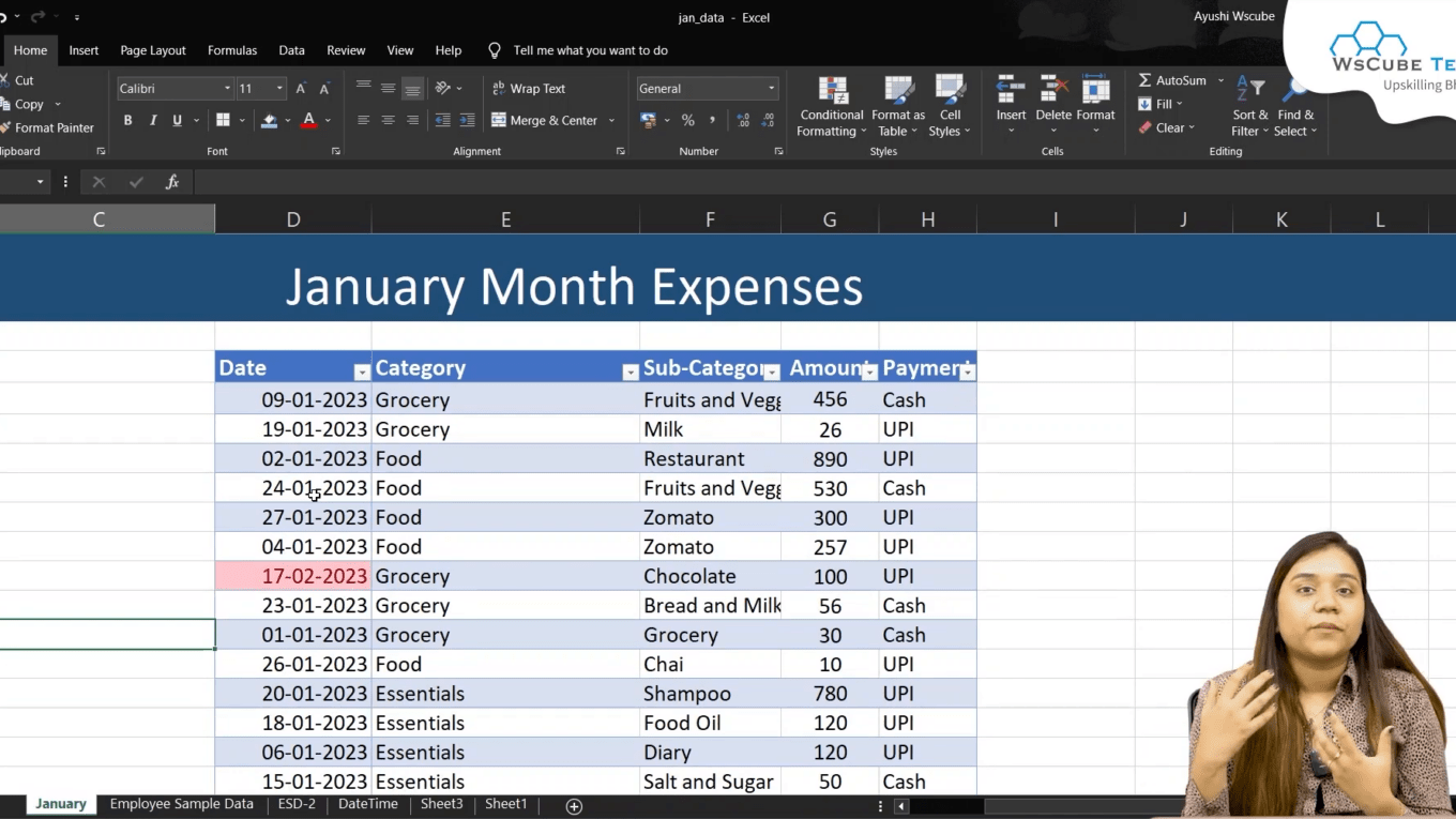
To highlight cells based on specific criteria, follow these steps:

1. Select the range of cells you want to format.
2. Navigate to the Home tab on the Ribbon.
3. Click on Conditional Formatting.
4. Choose Highlight Cells Rules and select your desired rule (e.g., Greater Than, Less Than).
5. Enter the value for the condition and choose the formatting style.
6. Click OK to apply the formatting.

2. Using Data Bars for Visual Representation 📊

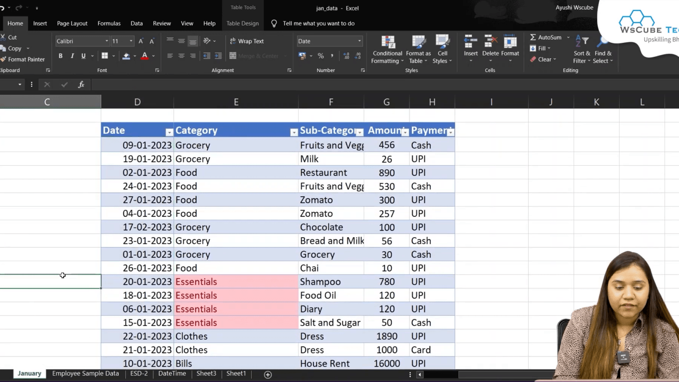
Data bars make it easy to visualize the magnitude of values in a range. Here’s how to add data bars:

1. Select the range of cells.
2. Go to the Home tab and click on Conditional Formatting.
3. Choose Data Bars and select a style.

Data bars will automatically adjust based on the values in the selected cells, providing an immediate visual cue of the data’s relative size.

Advanced Conditional Formatting Techniques 🔧

Once you are comfortable with the basics, you can explore more advanced techniques in conditional formatting. These techniques include using formulas for more complex conditions.

1. Using Formulas for Conditional Formatting 🧮

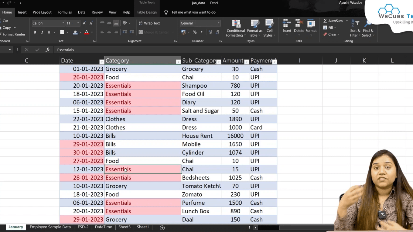
Formulas can be used to determine whether a cell should be formatted. Here’s how to apply conditional formatting using a formula:

1. Select the range of cells you want to format.
2. Go to Conditional Formatting and choose New Rule.
3. Select Use a formula to determine which cells to format.
4. Enter your formula (e.g., =A1>1000 for highlighting values greater than 1000).
5. Set the desired formatting and click OK.

2. Clearing Conditional Formatting 🔄

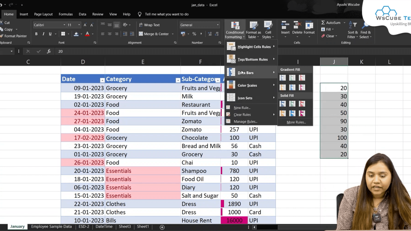
Sometimes, you may need to remove or clear conditional formatting. To do this:

1. Select the range of cells from which you want to clear formatting.
2. Go to Conditional Formatting.
3. Select Clear Rules and choose either Clear Rules from Selected Cells or Clear Rules from Entire Sheet.

Practical Applications of Conditional formatting with formulas 📈

Conditional formatting can be applied in various scenarios to enhance data analysis and visualization. Here are some practical applications:

• Budget Tracking: Highlight expenses that exceed a certain limit to keep your budget in check.
• Sales Performance: Use color scales to visualize sales trends over time.
• Project Management: Highlight overdue tasks based on deadlines.
• Inventory Management: Use icon sets to indicate stock levels (e.g., low, medium, high).

Common Mistakes to Avoid ❌

When using conditional formatting, it’s easy to make mistakes that can lead to confusion or misinterpretation of data. Here are some common pitfalls to avoid:

• Applying too many rules can overwhelm the data and make it harder to read.
• Using inconsistent formatting styles can lead to confusion.
• Not testing formulas can result in incorrect formatting.

Conclusion :Conditional formatting with formulas🎉

Conditional formatting is an essential tool in Excel that can enhance your data analysis capabilities. By understanding how to apply and customize conditional formatting, you can create visually appealing and informative spreadsheets that make it easier to interpret data. Whether you’re tracking sales, managing budgets, or analyzing performance, mastering conditional formatting will undoubtedly make you more efficient and effective in your data-related tasks.

For more tips and advanced techniques, continue exploring the features Excel has to offer, and don’t forget to practice regularly to sharpen your skills. Happy analyzing!